 Data Science
Pandas: Filtering and segmenting
This article is part of a series of practical guides for using the Python data processing library pandas. To see view all the available parts, click here.
One of the most common ways you will interact with a pandas DataFrame is by selecting different combinations of columns and rows. This can be done using the numerical positions of columns and rows in the DataFrame, column names and row indices, or by filtering the rows by applying some criteria to the data in the DataFrame. All of these options (and combinations of them) are available, so let’s dig in!
Reading in a dataset
If you don’t have a dataset you want to play around with, University of California Irvine has an excellent online repository of datasets that you can play with. For this explainer we are going to be using the Wine Quality dataset. If you want to follow along, you can import the dataset as follows:
import pandas as pd

df = pd.read_csv("https://archive.ics.uci.edu/ml/machine-learning-databases/wine-quality/winequality-red.csv", sep=';')
Selecting columns
Selecting columns in pandas is about as straight forward as it gets, but there are a few options worth covering. First, let’s keep it simple:
df['quality']

0       5
1       5
2       5
3       6
4       5
       ..
1594    5
1595    6
1596    6
1597    5
1598    6
Name: quality, Length: 1599, dtype: int64
By putting the name of the column we want to select inside square brackets and quotes (‘ and ” both work), we return a pandas Series. There is an alternative which returns the same results:
df.quality

0       5
1       5
2       5
3       6
4       5
       ..
1594    5
1595    6
1596    6
1597    5
1598    6
Name: quality, Length: 1599, dtype: int64
However, I recommend you do not use dot notation for several reasons:
- It will only work if the column name does not have any special characters. If, for example, your column name has a space in it (e.g.
'fixed acidity'), you won’t be able to use dot notation. - If your column name is the same as a DataFrame method name (e.g. you have a column called ‘sum’), using the dot notation will call the method instead of selecting the column.
- In more complicated scenarios you will often need to select columns dynamically. That is you will have column names that you store to a variable, then use that variable to access the column. This only works with the bracket notation.
What if we want to select multiple columns? Instead of passing one column name, we are going to pass a list of column names:
df[['fixed acidity', 'pH', 'quality']]

      fixed acidity    pH  quality
0               7.4  3.51        5
1               7.8  3.20        5
2               7.8  3.26        5
3              11.2  3.16        6
4               7.4  3.51        5
...             ...   ...      ...
1594            6.2  3.45        5
1595            5.9  3.52        6
1596            6.3  3.42        6
1597            5.9  3.57        5
1598            6.0  3.39        6

[1599 rows x 3 columns]
You might notice that we now have double square brackets. To understand why we need them, let’s reorganize our code a little:
columns_to_extract = ['fixed acidity', 'pH', 'quality']
df[columns_to_extract]
As this hopefully makes clearer, one set of square brackets is the syntax for selecting columns from a DataFrame in pandas, the other set is needed to create the list of column names.
What if we don’t know the column names or just want to select columns based on their position in the DataFrame rather than their name? Here we can use iloc or “integer-location”:
df.iloc[:, 0]

0        7.4
1        7.8
2        7.8
3       11.2
4        7.4
        ...
1594     6.2
1595     5.9
1596     6.3
1597     5.9
1598     6.0
Name: fixed acidity, Length: 1599, dtype: float64
To explain this syntax, first let’s understand what iloc does. iloc is a method for selecting rows and columns in a DataFrame, based on their zero-indexed integer location in the DataFrame. That is, the first column (counting from left to right) will be column 0, the second column will be 1, and so on. The same applies to the rows (counting from top to bottom), the first row is row 0, second is row 1 and so on. The full syntax for iloc is:
df.iloc[<row numbers>, <column numbers>]When we pass ":" to iloc before the "," as we did in the example above, we tell iloc to return all rows. If we passed ":" after the "," we would return all columns.
Now let’s combine a couple of these techniques. We can also pass lists of numbers for both the rows and columns to iloc. Before scrolling down, see if you can guess what the following will return:
df.iloc[[0, 1], [0, 1, 2]]…
…
…
…
If you guessed the first two rows for the first three columns, well done!
   fixed acidity  volatile acidity  citric acid
0            7.4              0.70          0.0
1            7.8              0.88          0.0
Selecting rows
When it comes to selecting or filtering rows in a DataFrame, there are typically two scenarios:
- We have a list of rows we want to select based on the index; or
- We want to filter based on the values in one or more columns.
By name
Let’s start with the less common use case as it is the simpler one to understand. Every DataFrame by default has an index. This index works like column names for rows: we can use it to select a row or a selection of rows. But first let’s look at the index for the DataFrame from earlier:
df.index

RangeIndex(start=0, stop=1599, step=1)
This output tells us that our index is just a list of sequential numbers from 0 to 1598. This aligns exactly with the zero-indexes numbered rows we were using with iloc earlier. However, to show they are different things, let’s create a new column called id that will be the current index plus 10, and then set that column as the index:
df['id'] = df.index + 10
df.set_index('id', inplace=True)

df.index

Int64Index([  10,   11,   12,   13,   14,   15,   16,   17,   18,   19,
            ...
            1599, 1600, 1601, 1602, 1603, 1604, 1605, 1606, 1607, 1608], dtype='int64', name='id', length=1599)
Now we can use this new index to select the first row of the DataFrame, which now has the index 10:
df.loc[10]

fixed acidity            7.4000
volatile acidity         0.7000
citric acid              0.0000
residual sugar           1.9000
chlorides                0.0760
free sulfur dioxide     11.0000
total sulfur dioxide    34.0000
density                  0.9978
pH                       3.5100
sulphates                0.5600
alcohol                  9.4000
quality                  5.0000
Name: 10, dtype: float64
We are now selecting the first row by index. You can also test by trying to select row 0 to confirm that there is no longer a row with that index.
Now let’s talk a little about loc. loc is the named equivalent to iloc, meaning that instead of passing it lists of zero-indexed row and column numbers, we pass it the names of columns and the indices of rows:
df.loc[<row indices>, <column names>]In practice, this ends up being much more useful than iloc. In fact, most experienced pandas users wouldn’t even have to take their socks off to count the number of times they’ve used iloc.
Something that is common to loc and iloc is that if we just want to select some rows for all columns, we don’t actually need to pass the columns at all. In other words df.loc[[10, 11, 12]] is the same as df.loc[[10, 11, 12], :].
By value
A very common use case is that we need to select a subset of rows based on the values in one or more columns. The way we do that is syntactically simple, but also very powerful once you understand what it is actually doing. Let’s start by looking at the syntax:
df[df['fixed acidity'] > 12]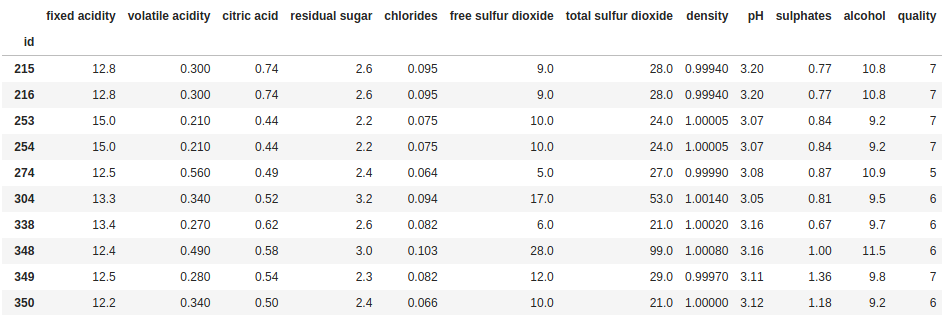
This line of code will return all rows in the DataFrame where the value in the “fixed acidity” column is greater than 12. But why do we need to repeat df? Let’s reorganize our code again for a bit of clarity:
filter = df['fixed acidity'] > 12
df[filter]
The key to understanding what the code is doing is understanding what filter in the above code is. When we run the first line of code above, filter becomes a Series (basically a list with some metadata) that has the same length as the DataFrame (i.e. one value for every row), and each value in that Series is either True or False. For our example, the value will be True where fixed acidity is greater than 12, and False otherwise. When we pass that list of True and False values to the DataFrame (or to loc), it will return the rows with a True value.
Why is this important to understand? Because it means you aren’t limited to generating a list of True and False values using the columns of the DataFrame you are working with. For example, I can generate a list of True and False values based on arbitrary things like whether the row number (not the index) is divisible by 3 (or in other words, selecting every third row):
every_3rd_row = [i % 3 == 0 for i in range(len(df))]
df[every_3rd_row]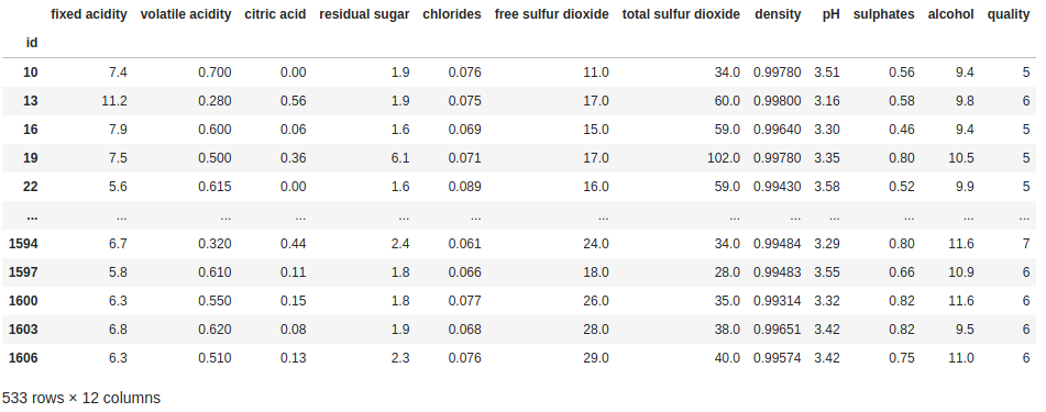
Obviously this is not something that you are likely to see used in practice, but the point is simply to show that once you understand that filters are just lists of True and False values, you are free to generate that list any way you want/need to.
Filtering a DataFrame for multiple conditions
What if we want to filter the DataFrame for multiple conditions? To do that, we are going going to need the following characters:
| Character | Meaning |
| & | AND condition |
| | | OR condition |
| ~ | negation |
Let’s look at an example:
filter = ((df["fixed acidity"] > 12) & (df["volatile acidity"] < 0.3)) | (df["quality"] == 3)
df[filter]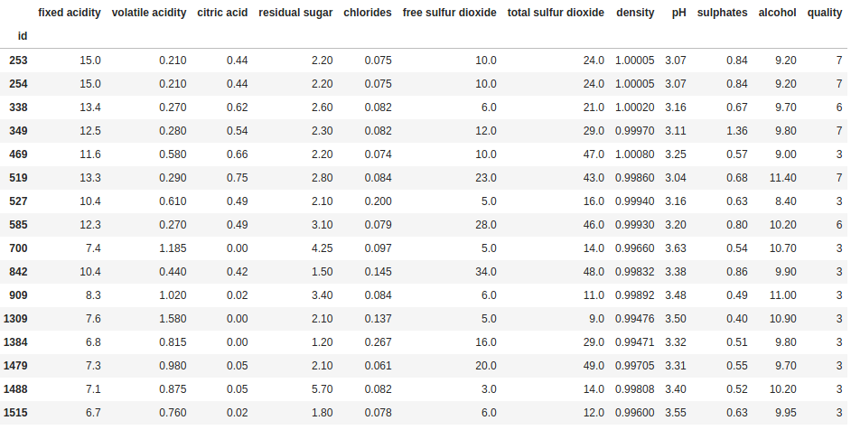
Using the same structure as before, separating out the filter from the line where we apply the filter to the DataFrame, we are now filtering for three conditions – “fixed acidity” has to be greater than 12 and “volatile acidity” has to be less than 0.3; or “quality” has to be equal to 3. Note that you can keep adding more and more conditions in the same way, you just need ensure to wrap each individual condition in parentheses “()”, and also use parentheses to specify how you want to group the conditions when you use an or condition.
There are lots of more advanced methods for creating these True/False series for filtering, but that is a subject for a separate explainer.
Selecting rows and columns
The above describes all the essential building blocks for how to filter and segment a DataFrame. We can select specific columns and we can filter the rows using multiple criteria. Now we just have to put it all together. This is where loc really shows its value; loc doesn’t just work with row indices, it also works with those lists of True and False values. So now we can combine those filters and a selection of column names:
filter = ((df["fixed acidity"] > 12) & (df["volatile acidity"] < 0.3)) | (df["quality"] == 3)
df.loc[filter, ["density", "pH"]]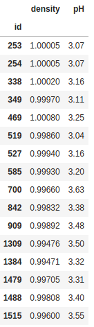
We also aren’t limited to just selecting these values, we can also use these selections to overwrite values. For example, let’s imagine I really like sweet red wines. Before I show these ratings to someone who is going to buy wines for me, I want to assign a quality of 9 to the wines with residual sugar in the the top 1%. Let’s see how this could be done:
cutoff = df["residual sugar"].quantile(0.99)
df.loc[df["residual sugar"] >= cutoff, "quality"] = 9
df.sort_values(["residual sugar", "quality"], ascending=False).head(20)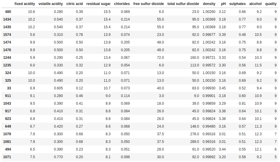
In the first line, we work out the cutoff point in terms of residual sugar and assign that value to a variable called cutoff. We use the loc method to filter the rows and select the column we want to update, then assign the new higher rating to everything that meets the criteria. Finally, we use sort_values to confirm it worked.
Wrapping up
In this explainer we have looked at a range of ways to filter the rows and columns of a DataFrame. This includes the loc and iloc methods, and how a list of True and False values, however it is created, can be used to filter the rows in a DataFrame. We also looked at how we can filter a DataFrame based on very complex criteria using combinations of simple building blocks and and (&), or (|) and negation (~) operators. With these tools, you will be able to filter and segment a DataFrame in practically anyway you are likely to need.