 Data Science
Pandas: Basic data interrogation
This article is part of a series of practical guides for using the Python data processing library pandas. To see view all the available parts, click here.
Once we have our data in a pandas DataFrame, the basic table structure in pandas, the next step is how do we assess what we have? If you are coming from Excel or R Studio, you are probably used to being able to look at the data any time you want. In python/pandas, we don’t have a spreadsheet to work with, and we don’t even have an equivalent of R Studio (although Jupyter notebooks are a similar concept), but we do have several tools available that can help you get a handle on what your data looks like.
DataFrame Dimensions
Perhaps the most basic question is how much data do I actually have? Did I successfully load in all the rows and columns I expected or are some missing? These questions can be answered with the shape method:
import pandas as pd

df = pd.read_csv("https://archive.ics.uci.edu/ml/machine-learning-databases/wine-quality/winequality-red.csv", sep=';')

print(df.shape)

(1599, 12)
shape returns a tuple (think of it as a list that you can’t alter) which tells you the number of rows and columns, 1599 and 12 respectively in this example. You can also use len to get the number of rows:
print(len(df))

1599
Using len is also slightly quicker than using shape, so if it is just the number of rows you are interested in, go with len.
Another dimension we might also be interested in is the size of the table in terms of disk space . For this we can use the memory_usage method:
print(df.memory_usage())

Index                     128
fixed acidity           12792
volatile acidity        12792
citric acid             12792
residual sugar          12792
chlorides               12792
free sulfur dioxide     12792
total sulfur dioxide    12792
density                 12792
pH                      12792
sulphates               12792
alcohol                 12792
quality                 12792
dtype: int64
This tells us the space, in bytes, each column is taking up on the disk. If we want to know the total size of the DataFrame, we can take a sum, and then to get the number into a more usable metric like kilobytes (kB) or megabytes (MB), we can divide by 1024 as many times as needed.
print(df.memory_usage().sum() / 1024)  # Size in kB

150.03125
Lastly, for these basic dimension assessments, we can generate a list of the data types of each column. This can be a very useful early indicator that your data has been read in correctly. If you have a column that you believe should be numeric (i.e. a float64 or an int64) but it is listed as object (pandas speak for categorical data), it may be a sign that something has not been interpreted correctly:
print(df.dtypes)

fixed acidity           float64
volatile acidity        float64
citric acid             float64
residual sugar          float64
chlorides               float64
free sulfur dioxide     float64
total sulfur dioxide    float64
density                 float64
pH                      float64
sulphates               float64
alcohol                 float64
quality                   int64
dtype: object
Viewing some sample rows
After we have satisfied ourselves that we have the expected volume of data in our DataFrame, we might want to look at some actual rows of data. Particularly for large datasets, this is where the head and tail methods come in handy. As the names suggest, head will return the first n rows of the DataFrame and tail will return the last n rows of the DataFrame (n is set to 5 by default for both).
print(df.head())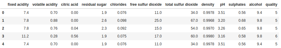
Aside from this basic use, we can use head and tail in some very useful ways with some alterations/additions. First off, we can set n to what ever value we want, showing as many or few rows as desired:
print(df.head(10))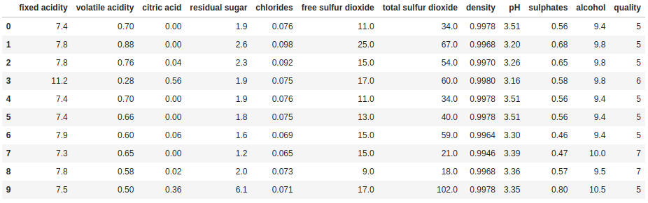
We can also combine it with sort_values to see the top (or bottom) n rows of data sorted by a column, or selection of columns:
print(df.sort_values('fixed acidity', ascending=False).head(10))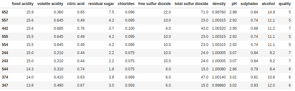
Finally, if we have a lot of columns, too many to display all of them in Jupyter or the console, we can combine head/tail with transpose to inspect all the columns for a few rows:
print(df.head().transpose())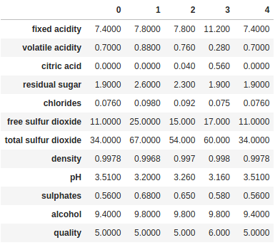
Summary Statistics
Moving on, the next step is typically some exploratory data analysis (EDA). EDA is a very open ended process so no one can give you an explicit set of instructions on how to do it. Each dataset is different and to a large extent, you just have to allow your curiosity to run wild. However, there are some tools we can take advantage of in this process.
Describe
The most basic way to summarize the data in your DataFrame is the describe method. This method, by default, gives us a summary of all the numeric fields in the DataFrame, including counts of values (which exclude null values), the mean, standard deviation, min, max and some percentiles.
df.describe()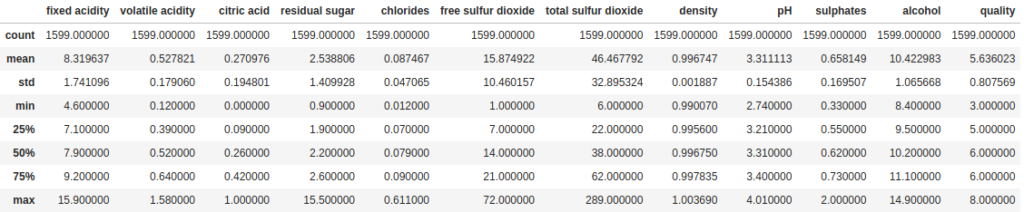
This is nice, but let’s talk about what isn’t being shown. Firstly, by default, any non-numeric and date fields are excluded. In the dataset we are using in this example we don’t have any non-numeric fields, so let’s add a couple of categorical fields (they will just have random letters in this case), and a date field:
import string
import random


df['categorical'] = [random.choice(string.ascii_letters) for i in range(len(df))]
df['categorical_2'] = [random.choice(string.ascii_letters) for i in range(len(df))]
df['date_col'] = pd.date_range(start='2020-11-01', periods=len(df))

df.describe()
As we can see, the output didn’t change. But we can use some of the parameters for describe to address that. First, we can set include='all' to include all datatypes in the summary:
df.describe(include='all')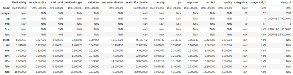
Now for the categorical columns it tells us some useful numbers about the number of unique values and which value is the most frequent. But the way it is handling the date column is like a categorical value. We can also change that so it treats it as numeric value by setting the datetime_as_numeric parameter to True:
df[['date_col]].describe(datetime_as_numeric=True)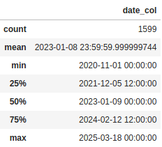
The pandas_summary Library
Building on top of the kind of summaries that are produced by describe, some very talented people have developed a library called pandas_summary. This library is purely designed to generate informative summaries of pandas DataFrames. First though we need to do some quick setup (you may need to install the library using pip):
from pandas_summary import DataFrameSummary

dfs = DataFrameSummary(df)
Now let’s take a look at two ways we can use this new DataFrameSummary object. The first one is columns_stats. This is similar to what we saw previously with describe, but with one useful addition: the number and percent of missing values in each column:
dfs.columns_stats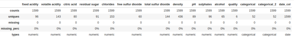
Secondly, my personal favorite, by selecting a column from we can look at an individual column to get some really detailed statistics, plus a histogram thrown in for numeric fields:
dfs['fixed acidity']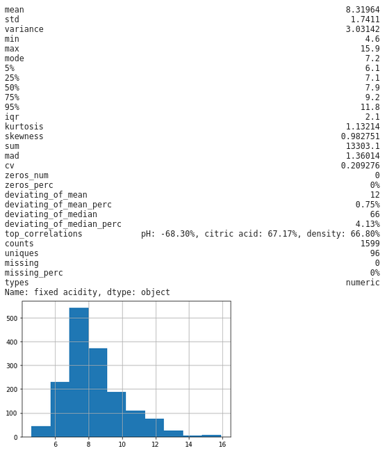
Seaborn
Seaborn is a statistical data visualization library for python with a full suite of charts that you should definitely look into if you have time, but for today we are going to look at just one very nice feature – pairplot. This function will generate a pairwise correlation plots for all the columns in your DataFrame with literally one line:
import seaborn as sns

sns.pairplot(df, hue="quality")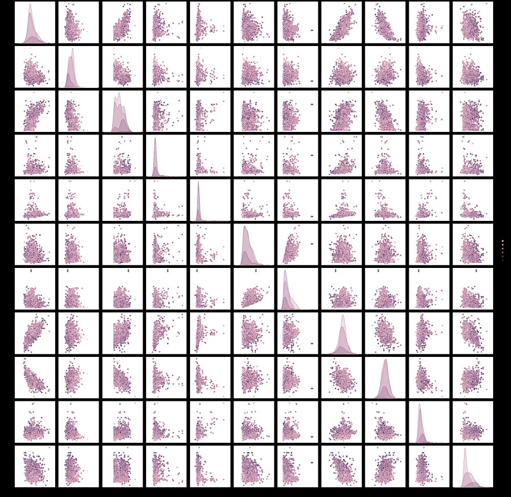
The colors of the plot will be determined by the column you select for the hue parameter. This allows you to see how the values in that column are impacted by the two features in each pairwise plot , but also along the axis where you would have a plot of a feature against itself, we get the distributions of that variable for different values in your hue column.
Note, if you have a lot of columns, be aware that this type of chart will become less useful, and will also likely take a lot of time to render.
Wrapping Up
Exploratory data analysis (EDA) should be an open ended and flexible process that never really ends. However, when we are first trying to understand the basic dimensions of a new dataset and what it contains, there are some common methods we can employ such as shape and describe and dtypes, and some very useful third party libraries such as pandas_summary and seaborn. While this explainer does not provide a comprehensive list of methods and techniques, hopefully it has provided you with somewhere to get started.